[ < ] [ > ]   [ << ] [ Up ] [ >> ]         [Top] [Contents] [Index] [ ? ]

8. Plotting


[ < ] [ > ]   [ << ] [ Up ] [ >> ]         [Top] [Contents] [Index] [ ? ]

8.1 Introduction to Plotting

Maxima uses an external plotting package to make the plots (see the section on Plotting Interfaces below). Maxima calculates set of points to be plotted and pass the to the plotting package together with a set of commands; the commands and plot data are passed to the external program either through a pipe or by saving them into a file with the extension maxout.interface, where interface is the name of the plotting interface being used.

The maxout.interface file, in the cases when it is used, is created in the directory specified by the variable temp_dir. That location can be changed; by assigning to that variable a string that represents a valid directory where Maxima can create new files.

After a plot has been obtained, the file maxout.interface can be executed again with the appropriate external program. If a Maxima plotting command fails to show anything, that file can be inspected to look for possible sources of problems.


[ < ] [ > ]   [ << ] [ Up ] [ >> ]         [Top] [Contents] [Index] [ ? ]

8.1.1 Plotting Interfaces

Currently, Maxima can one of two external plotting programs: Gnuplot or Xmaxima. There are various different interfaces for those programs, which can be selected with the option [plot_format,interface], where interface is one of the following:

·

@ref{Category: Plotting}


[ < ] [ > ]   [ << ] [ Up ] [ >> ]         [Top] [Contents] [Index] [ ? ]

8.2 Functions and Variables for Plotting

Function: contour_plot (expr, x_range, y_range, options, ...)

Plots the contours (curves of equal value) of expr over the region x_range by y_range. Any additional arguments are treated the same as in plot3d.

contour_plot only works when the plot format is gnuplot or gnuplot_pipes.

See also implicit_plot.

Examples:

(%i1) contour_plot (x^2 + y^2, [x, -4, 4], [y, -4, 4]);
(%o1) 
(%i2) contour_plot (sin(y) * cos(x)^2, [x, -4, 4], [y, -4, 4]);
(%o2) 
(%i3) F(x, y) := x^3 + y^2;
                                   3    2
(%o3)                  F(x, y) := x  + y
(%i4) contour_plot (F, [u, -4, 4], [v, -4, 4]);
(%o4) 
(%i5) contour_plot (F, [u, -4, 4], [v, -4, 4], [gnuplot_preamble,
      "set size ratio -1"]);
(%o5) 
(%i6) set_plot_option ([gnuplot_preamble,
                        "set cntrparam levels 12"])$

(%i7) contour_plot (F, [u, -4, 4], [v, -4, 4]);
·

@ref{Category: Plotting}

Option variable: in_netmath

Default value: false

When in_netmath is true, plot3d prints OpenMath output to the console if plot_format is openmath; otherwise in_netmath (even if true) has no effect. in_netmath has no effect on plot2d.

Function: plot2d (expr, x_range, ..., options, ...)
Function: plot2d ([expr_1, ..., expr_n], ..., options, ...)
Function: plot2d ([expr_1, ..., expr_n], x_range,..., options, ...)

Where expr, expr_1, ..., expr_n can be either expressions, or Maxima or Lisp functions or operators, or a list with the any of the forms: [discrete, [x1, ..., xn], [y1, ..., yn]], [discrete, [[x1, y1], ..., [xn, ..., yn]] or [parametric, x_expr, y_expr, t_range].

Displays a plot of one or more expressions as a function of one variable.

plot2d plots one expression expr or several expressions [name_1, ..., name_n]. The expressions that are not of the parametic or discrete types should all depend only on one variable var and it will be mandatory the use of x_range to name that variable and gives its minimum and maximum values, using the syntax: [variable, min, max]. The plot will show the horizontal axis bound by the values of min and max.

A expression to be plotted can also be given in the discrete or parametric forms. Namely, as a list starting with the word "discrete" or "parametric". The keyword discrete must be followed by two lists of values, both with the same length, which are the horizontal and vertical coordinates of a set of points; alternatively, the coordinates of each point can be put into a list with two values, and all the coordinates of the points should be inside another list. The keyword parametric must be followed by two expressions x_expr and y_expr, and a range of the form [param, min, max]. The two expressions must depend only on the parameter param, and the plot will show the path traced out by the point with coordinates (x_expr, y_expr) as param increases from min to max.

The range of the vertical axis is not mandatory. It is one more of the options for the command, with the syntax: [y, min, max]. If that option is used, the plot will show that entire range, even if the expressions do not reach all that range. Otherwise, if a vertical range is not specified by set_plot_option, the boundaries of the vertical axis will be set up automatically.

All other options should also be lists, starting with the name of the option. The option xlabel can be used to give a label for the horizontal axis; if that option is not used, the horizontal axis will be labeled with the name of the variable specified in x_range, or with the expression x_expr in the case of just one parametric expression, or it will be left blank otherwise.

A label for the vertical axis can be given with the ylabel option. If there is only one expression to be plotted and the ylabel option was not used, the vertical axis will be labeled with that expression, unless it is too large, or with the expression y_expr if the expression is parametric, or with the text "discrete data" if the expression is discrete.

The options [logx] and [logy] do not need any parameters. They will make the horizontal and vertical axes be scaled logarithmically.

If there are several expressions to be plotted, a legend will be written to identiy each of the expressions. The labels that should be used in that legend can be given with the option legend. If that option is not used, Maxima will create labels from the expressions.

By default, the expressions are plotted as a set of line segments joining adjacent points within a set of points which is either given in the discrete form, or calculated automatically from the expression given, using an algorithm that automatically adapts the steps among points using as an initial estimate of the total number of points the value set with the nticks option. The option style can be used to make one of the expressions to be represented as a set of isolated points, or as points and line segments.

There are several global options stored in the list plot_options which can be modified with the function set_plot_option; any of those global options can be overriden with options given in the plot2d command. There are also other options which are not part of the global options array plot_options and which can be given only as part of the plot2d command; those options are: logx, logy, box, legend, xlabel, ylabel, psfile and style.

A function to be plotted may be specified as the name of a Maxima or Lisp function or operator, a Maxima lambda expression, or a general Maxima expression. If specified as a name or a lambda expression, the function must be a function of one argument.

Examples:

Plots of common functions.

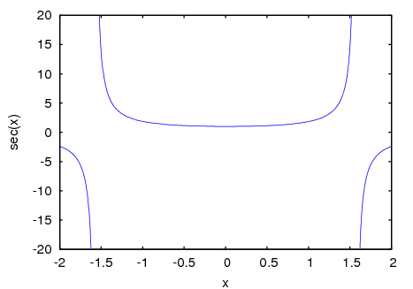
(%i1) plot2d (sin(x), [x, -5, 5])$

(%i2) plot2d (sec(x), [x, -2, 2], [y, -20, 20], [nticks, 200])$

figures/plotting2
figures/plotting3

Plotting functions by name.

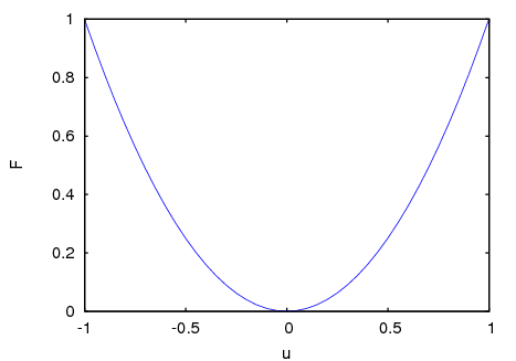
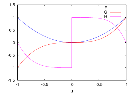
(%i3) F(x) := x^2 $

(%i4) :lisp (defun |$g| (x) (m* x x x))

$g
(%i5) H(x) := if x < 0 then x^4 - 1 else 1 - x^5 $

(%i6) plot2d (F, [u, -1, 1])$

(%i7) plot2d ([F, G, H], [u, -1, 1], [y, -1.5, 1.5])$

figures/plotting4
figures/plotting5

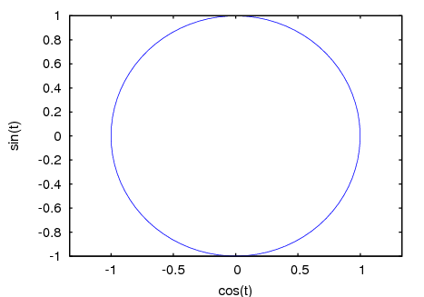
We can plot a circle using a parametric plot with a parameter t. It is not necessary to give a range for the horizontal range, since the range of the parameter t determines the domain. However, since the graph's horizontal and vertical axes lengths are in the 4 to 3 proportion, we will use the xrange option to obtain the same scaling in both axes:

(%i8) plot2d ([parametric, cos(t), sin(t), [t,-%pi,%pi],
      [nticks,80]], [x, -4/3, 4/3])$

figures/plotting6

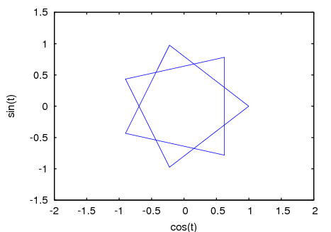
If we repeat that plot with only 8 points and extending the range of the parameter to give two turns, we will obtain the plot of a star:

(%i9) plot2d ([parametric, cos(t), sin(t), [t, -%pi*2, %pi*2],
        [nticks, 8]], [x, -2, 2], [y, -1.5, 1.5])$

figures/plotting7

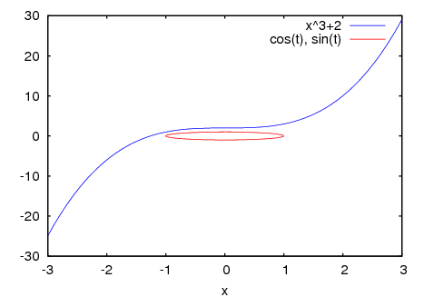
Combination of an ordinary plot of a cubic polynomial with a parametric plot of a circle:

(%i10) plot2d ([x^3+2, [parametric, cos(t), sin(t), [t, -5, 5],
        [nticks, 80]]], [x, -3, 3])$

figures/plotting8

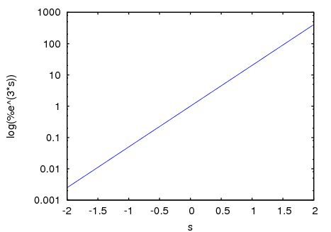
Example of a logarithmic plot:

(%i11) plot2d (exp(3*s), [s, -2, 2], [logy])$

figures/plotting9

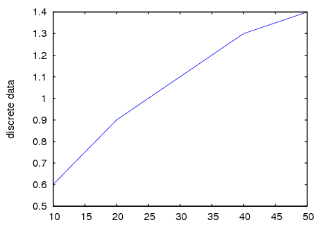
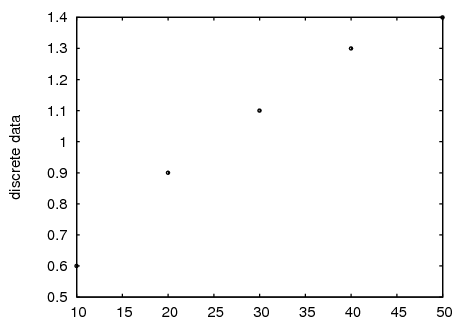
To show some examples of discrete plots, we will start by entering the coordinates of 5 points, in the two different ways that can be used:

(%i12) xx:[10, 20, 30, 40, 50]$
(%i13) yy:[.6, .9, 1.1, 1.3, 1.4]$
(%i14) xy:[[10,.6], [20,.9], [30,1.1], [40,1.3], [50,1.4]]$

To plot those data points, joined with line segments, we use:

(%i15) plot2d([discrete,xx,yy])$

figures/plotting10

We will now show the plot with only points, and illustrating the use of the second way of giving the points coordinates:

(%i16) plot2d([discrete, xy], [style, points])$

figures/plotting11

The plot of the data points can be shown together with a plot of the theoretical function that predicts the data:

(%i17) plot2d([[discrete,xy], 2*%pi*sqrt(l/980)], [l,0,50],
        [style, [points,5,2,6], [lines,1,1]],
        [legend,"experiment","theory"],
        [xlabel,"pendulum's length (cm)"], [ylabel,"period (s)"])$

figures/plotting12

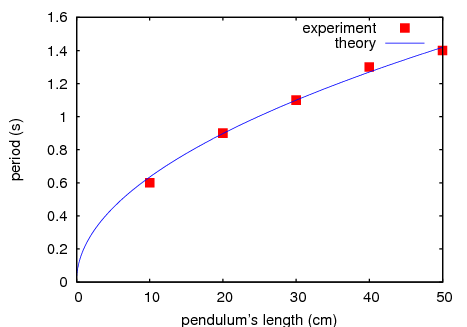
The meaning of the three numbers after the "points" style option are as follows; 5: radius of the points, 2: index of color used (red), 6: type of objects used (solid squares). The two numbers after the "lines" style option give the thickness of the line (1 point) and the color (1 corresponds to blue).

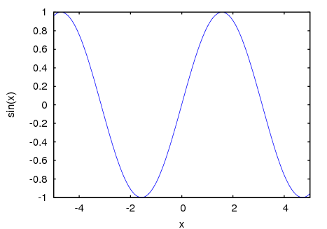
To save a plot of sin(x) to the file sin.ps, one can use:

(%i18) plot2d (sin(x), [x, 0, 2*%pi], [psfile, "sin.eps"])$

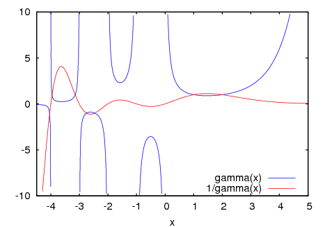
The next example uses the y option to chop off singularities and the gnuplot_preamble option to put the key at the bottom of the plot instead of the top.

(%i19) plot2d ([gamma(x), 1/gamma(x)], [x, -4.5, 5], [y, -10, 10],
                     [gnuplot_preamble, "set key bottom"])$

figures/plotting14

We can also use a gnuplot_preamble to produce fancy x-axis labels. (Note that the gnuplot_preamble string must be entered without any line breaks.)

(%i20) my_preamble: "set xtics ('-2pi' -6.283, \
'-3pi/2' -4.712, '-pi' -3.1415, '-pi/2' -1.5708, '0' 0, \
'pi/2' 1.5708, 'pi' 3.1415,'3pi/2' 4.712, '2pi' 6.283)"$

(%i21) plot2d([cos(x), sin(x), tan(x), cot(x)],
       [x, -2*%pi, 2.1*%pi], [y, -2, 2], [axes, x]
       [gnuplot_preamble, my_preamble]);

figures/plotting15

This example uses a gnuplot_preamble to produce fancy x-axis labels, and produces PostScript output that takes advantage of the advanced text formatting available in gnuplot. (Note that the gnuplot_preamble string must be entered without any line breaks.)

(%i22) my_preamble: "set xtics ('-2{/Symbol p}' \
-6.283, '-3{/Symbol p}/2' -4.712, '-{/Symbol p}' -3.1415, \
'-{/Symbol p}/2' -1.5708, '0' 0,'{/Symbol p}/2' 1.5708, \
'{/Symbol p}' 3.1415,'3{/Symbol p}/2' 4.712, '2{/Symbol p}' \
6.283)"$

(%i23) plot2d ([cos(x), sin(x), tan(x)], [x, -2*%pi, 2*%pi],
    [y, -2, 2], [gnuplot_preamble, my_preamble],
    [psfile, "trig.eps"]);

See also plot_options, which describes plotting options.

·

@ref{Category: Plotting}

Function: xgraph_curves (list)

graphs the list of `point sets' given in list by using xgraph. If the program xgraph is not installed, this command will fail.

A point set may be of the form

[x0, y0, x1, y1, x2, y2, ...]

or

[[x0, y0], [x1, y1], ...]

A point set may also contain symbols which give labels or other information.

xgraph_curves ([pt_set1, pt_set2, pt_set3]);

graph the three point sets as three curves.

pt_set: append (["NoLines: True", "LargePixels: true"],
                          [x0, y0, x1, y1, ...]);

would make the point set (and subsequent ones), have no lines between points, and to use large pixels. See the man page on xgraph for more options to specify.

pt_set: append ([concat ("\"", "x^2+y")], [x0, y0, x1, y1, ...]);

would make there be a "label" of "x^2+y" for this particular point set. The " at the beginning is what tells xgraph this is a label.

pt_set: append ([concat ("TitleText: Sample Data")], [x0, ...])$

would make the main title of the plot be "Sample Data" instead of "Maxima Plot".

To make a bar graph with bars which are 0.2 units wide, and to plot two possibly different such bar graphs:

(%i1) xgraph_curves ([append (["BarGraph: true", "NoLines: true",
      "BarWidth: .2"], create_list ([i - .2, i^2], i, 1, 3)),
      append (["BarGraph: true", "NoLines: true", "BarWidth: .2"],
      create_list ([i + .2, .7*i^2], i, 1, 3))]);

figures/plotting13

A temporary file `xgraph-out' is used.

·

@ref{Category: Plotting}

System variable: plot_options

Elements of this list state the default options for plotting. If an option is present in a plot2d or plot3d call, that value takes precedence over the default option. Otherwise, the value in plot_options is used. Default options are assigned by set_plot_option. There are other local options specific to each plotting command, and not included in this list of global options.

Each element of plot_options is a list of two or more items. The first item is the name of an option, and the remainder comprises the value or values assigned to the option. In some cases the, the assigned value is a list, which may comprise several items.

The plot options which are recognized by plot2d and plot3d are the following:

Gnuplot options:

There are several plot options specific to gnuplot. Some of these options are raw gnuplot commands, specified as strings. Refer to the gnuplot documentation for more details. In most cases, these options can be replaced by one of the more general options above; in those cases we recommend that you use the most general form.

·

@ref{Category: Plotting}

Function: plot3d ([expr_1, expr_2, expr_3], x_range, y_range, ..., options, ...)
Function: plot3d (expr, x_range, y_range, ..., options, ...)
Function: plot3d (name, x_range, y_range, ..., options, ...)
Function: plot3d ([expr_1, expr_2, expr_3], x_rge, y_rge)
Function: plot3d ([name_1, name_2, name_3], x_range, y_range, ..., options, ...)

Displays a plot of one or three expressions as functions of two variables.

(%i1) plot3d (2^(-u^2 + v^2), [u, -3, 3], [v, -2, 2]);

figures/plotting19

plots z = 2^(-u^2+v^2) with u and v varying in [-3,3] and [-2,2] respectively, and with u on the x axis, and v on the y axis.

The same graph can be plotted using openmath (if Xmaxima is installed):

(%i2)  plot3d (2^(-u^2 + v^2), [u, -3, 3], [v, -2, 2],
               [plot_format, openmath]);

figures/plotting25

in this case the mouse can be used to rotate the plot to look at the surface from different sides.

An example of the third pattern of arguments is

(%i3) plot3d ([cos(x)*(3 + y*cos(x/2)), sin(x)*(3 + y*cos(x/2)),
   y*sin(x/2)], [x, -%pi, %pi], [y, -1, 1], ['grid, 50, 15]);

figures/plotting20

which plots a Moebius band, parametrized by the three expressions given as the first argument to plot3d. An additional optional argument ['grid, 50, 15] gives the grid number of rectangles in the x direction and y direction.

The function to be plotted may be specified as the name of a Maxima or Lisp function or operator, a Maxima lambda expression, or a general Maxima expression. In the form plot3d (f, ...) where f is the name of a function or a lambda expression, the function must be a function of two arguments. In the form plot3d ([f_1, f_2, f_3], ...) where f_1, f_2, and f_3 are names of functions or lambda expressions, each function must be a function of three arguments.

This example shows a plot of the real part of z^1/3, using polar coordinates. The options box and legend were also used to suppress the title and the axes box.

(%i4) plot3d (r^.33*cos(th/3), [r, 0, 1], [th, 0, 6*%pi],
      ['grid, 12, 80], ['transform_xy, polar_to_xy],
      [box, false],[legend,false]);

figures/plotting21

Other examples are the Klein bottle:

(%i5) expr_1: 5*cos(x)*(cos(x/2)*cos(y) + sin(x/2)*sin(2*y)
      + 3.0) - 10.0$
(%i6) expr_2: -5*sin(x)*(cos(x/2)*cos(y) + sin(x/2)*sin(2*y)
      + 3.0)$
(%i7) expr_3: 5*(-sin(x/2)*cos(y) + cos(x/2)*sin(2*y))$

(%i8) plot3d ([expr_1, expr_2, expr_3], [x, -%pi, %pi],
      [y, -%pi, %pi], ['grid, 40, 40]);

figures/plotting22

and a torus:

(%i9) expr_1: cos(y)*(10.0+6*cos(x))$
(%i10) expr_2: sin(y)*(10.0+6*cos(x))$
(%i11) expr_3: -6*sin(x)$
(%i12) plot3d ([expr_1, expr_2, expr_3], [x, 0, 2*%pi],
       [y, 0, 2*%pi], ['grid, 40, 40]);

figures/plotting23

Sometimes it is necessary to define a function to plot the expression. All the arguments to plot3d are evaluated before being passed to plot3d, and so trying to make an expression which does just what is needed may be difficult, and it is just easier to make a function.

(%i13) M: matrix([1, 2, 3, 4], [1, 2, 3, 2], [1, 2, 3, 4],
       [1, 2, 3, 3])$
(%i14) f(x, y) := float (M [?round(x), ?round(y)])$
(%i15) plot3d (f, [x, 1, 4], [y, 1, 4], ['grid, 4, 4])$

figures/plotting24

Here is a three-dimensional plot using the gnuplot pm3d terminal.

(%i7) plot3d (atan (-x^2 + y^3/4), [x, -4, 4], [y, -4, 4],
        [grid, 50, 50], [gnuplot_pm3d, true])$

figures/plotting16

And a three-dimensional plot without a mesh and with contours projected on the bottom plane. (Note that the gnuplot_preamble string must be entered without any line breaks.)

(%i8) my_preamble: "set pm3d at s;unset surface;set contour;\
set cntrparam levels 20;unset key"$
(%i9) plot3d(atan(-x^2 + y^3/4), [x, -4, 4], [y, -4, 4],
    [grid, 50, 50], [gnuplot_pm3d, true],
    [gnuplot_preamble, my_preamble])$

figures/plotting17

Finally, a plot where the z-axis is represented by color only.

(%i10) plot3d (cos (-x^2 + y^3/4), [x, -4, 4], [y, -4, 4],
    [gnuplot_preamble, "set view map; unset surface"],
    [gnuplot_pm3d, true], [grid, 150, 150])$

figures/plotting18

See the available options in plot_options.

·

@ref{Category: Plotting}

Function: make_transform (vars, fx, fy, fz)

Returns a function suitable for the transform function in plot3d. Use with the plot option transform_xy.

make_transform ([r, th, z], r*cos(th), r*sin(th), z)$

is a transformation to polar coordinates.

·

@ref{Category: Plotting}

Function: set_plot_option (option)

Assigns one of the global variables for plotting. option is specified as a list of two or more elements, in which the first element is one of the keywords on the plot_options list.

set_plot_option evaluates its argument and returns the complete list plot_options (after modifying one of its elements).

See also plot_options, plot2d, and plot3d.

Examples:

Modify the grid and x values. When a plot_options keyword has an assigned value, quote it to prevent evaluation.

(%i1) set_plot_option ([grid, 30, 40]);
(%o1) [[x, - 1.755559702014E+305, 1.755559702014E+305], 
[y, - 1.755559702014E+305, 1.755559702014E+305], [t, - 3, 3], 
[grid, 30, 40], [transform_xy, false], [run_viewer, true], 
[plot_format, gnuplot], [gnuplot_term, default], 
[gnuplot_out_file, false], [nticks, 10], [adapt_depth, 10], 
[gnuplot_pm3d, false], [gnuplot_preamble, ], 
[gnuplot_curve_titles, [default]], 
[gnuplot_curve_styles, [with lines 3, with lines 1, 
with lines 2, with lines 5, with lines 4, with lines 6, 
with lines 7]], [gnuplot_default_term_command, ], 
[gnuplot_dumb_term_command, set term dumb 79 22], 
[gnuplot_ps_term_command, set size 1.5, 1.5;set term postscript #
eps enhanced color solid 24]]
(%i2) x: 42;
(%o2)                          42
(%i3) set_plot_option (['x, -100, 100]);
(%o3) [[x, - 100.0, 100.0], [y, - 1.755559702014E+305, 
1.755559702014E+305], [t, - 3, 3], [grid, 30, 40], 
[transform_xy, false], [run_viewer, true], 
[plot_format, gnuplot], [gnuplot_term, default], 
[gnuplot_out_file, false], [nticks, 10], [adapt_depth, 10], 
[gnuplot_pm3d, false], [gnuplot_preamble, ], 
[gnuplot_curve_titles, [default]], 
[gnuplot_curve_styles, [with lines 3, with lines 1, 
with lines 2, with lines 5, with lines 4, with lines 6, 
with lines 7]], [gnuplot_default_term_command, ], 
[gnuplot_dumb_term_command, set term dumb 79 22], 
[gnuplot_ps_term_command, set size 1.5, 1.5;set term postscript #
eps enhanced color solid 24]]
·

@ref{Category: Plotting}


[ < ] [ > ]   [ << ] [ Up ] [ >> ]         [Top] [Contents] [Index] [ ? ]

8.2.1 Functions for working with the gnuplot_pipes format

Function: gnuplot_start ()

Opens the pipe to gnuplot used for plotting with the gnuplot_pipes format. Is not necessary to manually open the pipe before plotting.

·

@ref{Category: Plotting}

Function: gnuplot_close ()

Closes the pipe to gnuplot which is used with the gnuplot_pipes format.

·

@ref{Category: Plotting}

Function: gnuplot_restart ()

Closes the pipe to gnuplot which is used with the gnuplot_pipes format and opens a new pipe.

·

@ref{Category: Plotting}

Function: gnuplot_replot ()
Function: gnuplot_replot (s)

Updates the gnuplot window. If gnuplot_replot is called with a gnuplot command in a string s, then s is sent to gnuplot before reploting the window.

·

@ref{Category: Plotting}

Function: gnuplot_reset ()

Resets the state of gnuplot used with the gnuplot_pipes format. To update the gnuplot window call gnuplot_replot after gnuplot_reset.

·

@ref{Category: Plotting}


[ << ] [ >> ]           [Top] [Contents] [Index] [ ? ]

This document was generated by root on July, 13 2009 using texi2html 1.76.